Notes on dynamic programming - part 1

(This post is part of the dynamic programming series.)

These notes are based on the content of Introduction to the Design and Analysis of Algorithms (3rd Edition).

def: dynamic programming

A technique for solving problems with overlapping subproblems.

Instead of solving overlapping subproblems again and again, store the results in a table.

Ex: Fibonacci Sequence

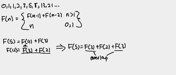
It's easy to see how the Fibonacci sequence spirals out of control in terms of subproblem overlap. The algorithm ends up recalculating various F(x)'s over and over again, as seen in the F(5) example above.

With dynamic programming, instead of recalculating known F(n) for n we've already seen, we store F(n) in some form of table and look up the value when needed.

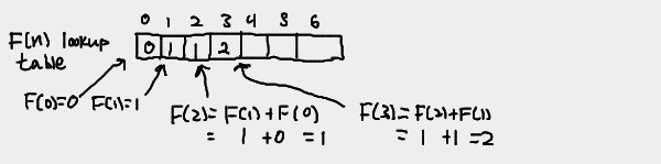
We can use an array to store the values of F(n) as we go. Consequently, the n-th element of the array is equal to F(n). Instead of substituting backwards from F(n) like in most recurrences, we start from F(0) and make our way up to F(n).

You could also avoid the overhead of an array by just keeping track of the last two numbers in the sequence.

Other examples of dynamic programming

Computing binomial coefficients
Constructing an optimal binary search tree (based on probabilities)
Warshall's algorithm for transitive closure
Floyd's algorithm for all-pairs shortest paths
Some instances of difficult discrete optimization problems

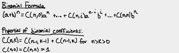
Computing a binomial coefficient

def: binomial coefficient

A binomial coefficient C(n,k) is the total number of combinations of k elements from an n-elemnt set, with 0 <= k <= n. This is also known as "n choose k"

We can store the values of the recurrence C(n,k) in a table like so:

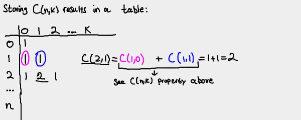
Note that this forms Pascal's Triangle!

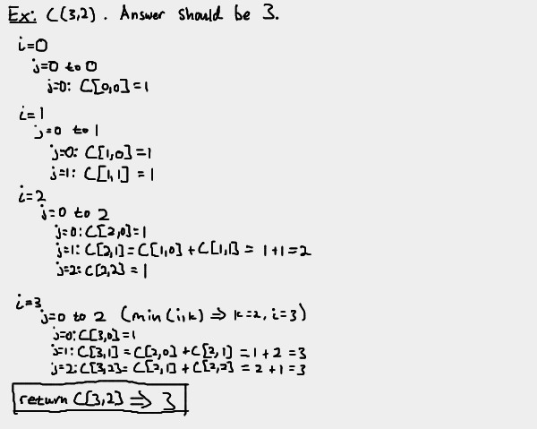
Here's an example where we solve C(5,2)

If we were to look at Pascal's Triangle, the intersection of row n=5 and column k=2 (both 0-indexed) has the value 10. You can look up any of the other C(n,k) values calculated above, and you'll find they are properly positioned on Pascal's Triangle.

Pseudocode

The pseudocode for finding C(n,k)

def binomial(n,k)
    for i=0 to n do
        for j=0 to min(i,k) do
            if j == 0 or j == i
                C[i,j] = 1
            else
                C[i,j] = C[i-1, j-1] + C[i-1, j]
    return C[n,k]

Algorithm hand-trace

A Python implementation

def binomial(n,k):
    C = []
    i = 0
    x = 0
    while i <= n:
        j = 0
        C.insert(i, [])
        while j <= min(i,k):
            if j == 0 or j == i:
                C[i].insert(j, 1)
            else:
                C[i].insert(j, C[i-1][j-1] + C[i-1][j])
            j += 1
            x += 1
        i += 1
    print("Number of additions: %d" % x)
    return C[n][k]

print(binomial(5,2)) # 10

raw source

Analysis

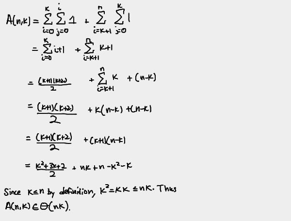
The basic operation is addition, which occurs once each time the inner loop is executed. The algorithm essentially has two "stages". In the first stage, we have i<k. This means min(i,k)==i, so the inner loop gets executed i times for each iteration of i while i=<k. Once i>k, though, min(i,k)==k, so the inner loop gets executed k times for each iteration of i while i<=n. Since a single addition occurs for each execution of the inner loop, we now have all the information we need to come up with a formula for the number of additions performed by our binomial(n,k) algorithm.

Here are a few example tables produced by various calls to binomial(n,k). Pay close attention to the shape of the tables.

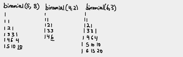
Could you find the pattern of the shapes?

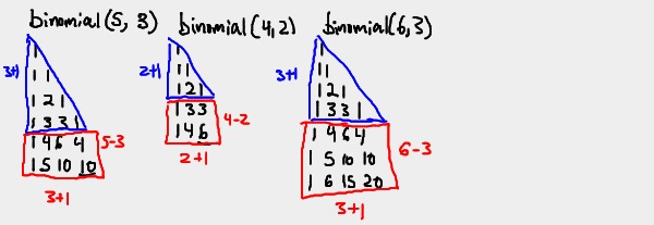
Each table is split into two shapes: A triangle with height k+1, and a rectangle with height n-k and width k+1. This is a direct result of the "stages" of the algorithm described above. Now that we have a higher understand of how our algorithm builds the table, we can now come up with a summation for the number of additions executed by binomial(n,k),

Warshall's algorithm: transitive closure

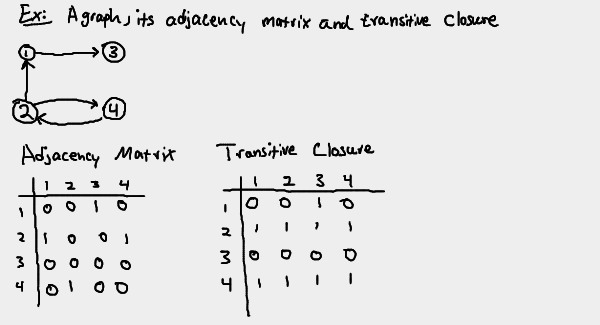
def: adjacency matrix

The adjacency matrix A = {a_ij} of a directed graph is the boolean matrix that has 1 in its i-th row and j-th column iff there is a directed edge from the i-th vertex to the j-th vertex.

def: transitive closure

The transitive closure of a directed graph with n vertices is an n x n boolean matrix T = {t_ij}, where the element in the i-th row and j-th column is 1 if there exists a nontrivial path from the i-th vertex to the j-th vertex, and is 0 otherwise.

Example:

Generating the transitive closure

We can naively generate the transitive closure of a digraph by doing a depth-first or breadth-first traversal starting from every vertex. This introduces a lot of overlap. Warshall's algorithm rectifies this problem by constructing the transitive closure through a series of nxnmatrices (with the assumption that the digraph's vertices are numbered from 1 to n.)

The series is as follows:

R⁽⁰⁾,...R^(k-1),R^(k),...R⁽ⁿ⁾

The element r_ij^(k) is located at the i-th row and j-th column of the matrix R^(k), with i,j = 1,2,...,n and k=0,1,...,n. This element is equal to 1 iff there is a nontrivial path from the i-th vertex to the j-th vertex with each intermediate vertex intermediate vertex (if any) numbered less than or equal to k.

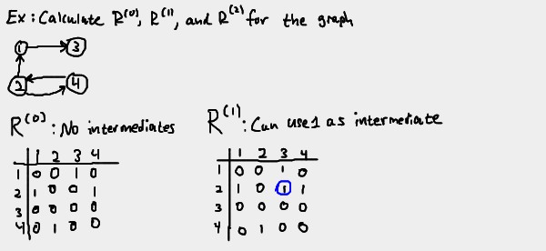
Since the vertices are numbered 1 to n, elements of R⁽⁰⁾ equal 1 iff there is a nontrivial path from the i-th vertex to the j-th vertex with no intermediate vertices. This is the same thing as the adjacency matrix.

Elements of R⁽¹⁾ equal 1 iff there is a nontrivial path from the i-th vertex to the j-th vertex, with the vertex 1 allowed as an intermediate.

Elements of R⁽²⁾ equal 1 iff there is a nontrivial path from the i-th vertex to the j-th vertex, with vertices 1 and 2 allowed as intermediates.

And so on.

As the `k in R^(k) increases, we have fewer "restrictions" on what vertices we can use as intermediates. Thus, we can expect each subsequent matrix in the series to have more 1's.

R⁽ⁿ⁾ is the transitive closure.

Example:

Notice how all the elements that are 1's in R⁽⁰⁾ are 1's in R⁽¹⁾. Similarly, all the elements that are 1's in R⁽¹⁾ are 1's in R⁽²⁾. We can actually compute all elements of each matrix R^(k) from its immediate predecessor R^(k-1)

Relating the matrices in the series

So how exactly can we relate R^(k) to R^(k-1)? Here's how.

Let r_ij^(k) = 1. By how we've defined R(k), this means there exists a nontrivial path from the i-th vertex v_i to the j-th vertex v_j, with all intermediate vertices <= k. Let L be this list of intermediate vertices. We can thus describe the path from v_i to v_j as

v_i, L, v_j

There are two possible scenarios from this point.

First scenario

In the first scenario, the k-th vertex, v_k, is not in the list of intermediate vertices L. Since all vertices in L are less than or equal to k but k is not in L, all vertices in L are less than or equal to k-1. So we have a path v_i, L, v_j with all vertices in L less than or equal to k-1. These conditions are sufficient to conclude that r_ij^(k-1) = 1.

Second scenario

In the second scenario, the k-th vertex, v_k, is in the list of intermediate vertices L. We can assume v_k only occurs once in L. If v_k does actually appear more than once in L, we can simply reconstruct the list to meet our requirements by eliminating all vertices between the first and last occurrences of v_k.

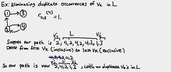
So now we once again have v_i, L, v_j. But now that we know v_k appears only once in L, we can separate L out into three groups: vertices before v_k, v_k, and vertices after v_k. We'll label the "before" group L1 and the "after" group L2. So now our path from v_i to v_j looks like

v_i, L1, v_k, L2, v_j

Since both L1 and L2 do not have v_k in them, we can conclude that all vertices in L1 and L2 are less than or equal to k-1.

With this information about the path and its vertices, we can make some conclusions.

We know there exists a path from v_i to v_k with each intermediate vertex less than or equal to k-1. By definition, this means r_ik^(k-1)=1. Similarly, we know r_kj^(k-1)=1.

What we've shown

Ultimately, we've shown that if r_ij^(k)=1, then either r_ij^(k-1)=1 (if v_k not in L) or both r_ik^(k-1)=1 and r_kj^(k-1)=1

The converse of these statements is also true, although the text does not explicitly prove it. This means we finally have an algorithm.

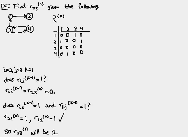
Algorithm

If a element r_ij is 1 in R^(k-1), it remains 1 in R^(k). If r_ij is 0 in R^(k-1), we change it to 1 in R^(k) iff r_ik^(k-1) and r_kj^(k-1) are both 1.

Example:

Pseudocode

# A: adjacency matrix of a digraph with n vertices
def warshall(A[1..n, 1..n]):
    R[0] = A
    for k=1 to n do
        for i = 1 to n do
            for j = 1 to n do
                R[k][i][j] = R[k-1][i][j] OR (R[k-1][i][k] AND R[k-1][k][j])
    return R[n]

Python implementation

The biggest issue porting the pseudocode over to Python was adjusting the algorithm to work with 0-index arrays. k still needs to start at 1 since R[0] is immediately assigned the adjacency matrix. The outermost loop needs to loop exactly n times with k starting at 1, so k<=n is the appropriate while condition. The inner loops need to loop exactly n times starting with their respective counters at 0 (for array indexing purposes), so var <= n-1 is the appropriate while condition for the inner loops.

The most confusing issue was how to treat k. When using k as part of an array index for a row/column, you have to subtract 1 to account for the 0-index. However, when referring to the k-th matrix, we don't adjust k since R was already defined as a 0-index array in the pseudocode.

def warshall(A, n):
    R = []
    R.insert(0, A)
    k = 1
    while k <= n:
        R.insert(k, [])
        i = 0
        while i <= n-1:
            R[k].insert(i, [])
            j = 0
            while j <= n-1:
                hasPath = R[k-1][i][j] or (R[k-1][i][k-1] and R[k-1][k-1][j])
                R[k][i].insert(j, int(hasPath))
                j += 1
            i += 1
        k += 1
    return R[n]



# Adjacency matrix of the graph used through the examples in the notes.
adj = [
    [0,0,1,0],
    [1,0,0,1],
    [0,0,0,0],
    [0,1,0,0],
]

print(warshall(adj, 4))

raw source

Analysis

The time efficiency of Warshall's algorithm is O(n³). Traversal based approaches for finding the transitive closure outperform Warshall's algorithm for sparse graphs represented by adjacency lists.

In regards to space efficiency, it's actually unnecessary to store so many matrices. Similar to the Fibonacci sequence and other dynamic programming problems, we can avoid the storage overhead of holding on to so many data structures.

Next time

Next time, we'll apply dynamic programming concepts to weighted graphs. We'll learn how to find the shortest path between two vertices in a graph using Floyd's Algorithm.