(This post is part of the dynamic programming series.)

These notes are based on the content of Introduction to the Design and Analysis of Algorithms (3rd Edition).

The ideas behind Warshall's algorithm, which was discussed in the previous notes on dynamic programming, can be applied to the more general problem of finding lengths of shortest paths in weighted graphs.

def: weighted graph

A graph which associates a label (called a weight) with every edge in the graph.

Example:

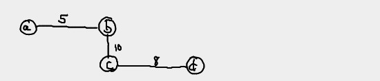
def: all-pairs shortest-path problem

Given a weighted connected graph, find the distances from each vertex to all other vertices.

Shortest-path algorithms play important parts in

• communications
• transportation networks
• operations research
• motion planning in video games

def: length of a path

The length of a path of a weighted graph is the accumulation of the weights of all the edges in the path.

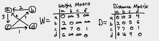
def: weight matrix

The distance matrix is an n x n matrix W. The element w_ij in the i-th row and j-th column of the matrix indicates the weight of the edge from the i-th vertex to the j-th vertex.

def: distance matrix

The distance matrix is an n x n matrix D. The element d_ij in the i-th row and j-th column of the matrix indicates the length of the shortest path from the i-th vertex to the j-th vertex.

def: shortest path

The shortest path from v_i to v_j is the path from v_i to v_j with the smallest length. In other words, it is the path with the lowest sum of all the edges in the path.

Note that the distance from a vertex to itself is 0. For the weight matrix W, the distance from a vertex A to a vertex B is infinity if there is no edge from vertex A to vertex B. For directed graphs, remember that an edge from A to B does not mean there is also an edge from B to A. That is why w_ab is infinity while w_ba is 2. That is not the case with undirected graphs, where the edge from A to B is by definition equal to the edge from B to A.

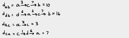
For the distance matrix D, the value of d_ij is the length of the path from the vertex i to the vertex j. Here are some examples to demonstrate how we filled out the distance matrix table.

The distance matrix can be generated with an algorithm that is similar to Warshall's algorithm. It's called Floyd's algorithm.

Floyd's algorithm

Floyd's algorithm computes the distance matrix of a weighted graph with n vertices through a series of nxn matrices (with the assumption that the graph's vertices are numbered from 1 to n.)

D⁽⁰⁾,...D^(k-1),D^(k),...D⁽ⁿ⁾

The algorithm works for digraphs and undirected graphs, but the graphs must not contain a negative cycle. Note how familiar the series above is to that of Warshall's algorithm.

def: negative cycle

A cycle whose edges sum to a negative value

The element d_ij^(k) is located at the i-th row and j-th column of the matrix D^(k) in the series, with i,j=1,2,...,n and k=0,1,...,n . This element is equal to the length of the shortest possible path from the i-th vertex to the j-th vertex, with all intermediate vertices less than or equal to k.

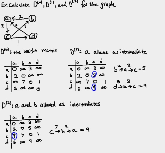
Since the vertices are numbered 1 to n, elements of D⁽⁰⁾, which are of the form d_ij⁽⁰⁾, are equal to the length of the shortest path from the i-th vertex to j-th vertex, with no intermediates allowed. This is exactly the same thing as the weight matrix.

Elements of D⁽¹⁾, which are of the form d_ij⁽¹⁾, are equal to the length of the shortest path from the i-th vertex to the j-th vertex with the vertex 1 allowed as an intermediate.

Elements of D⁽²⁾, which are of the form d_ij⁽²⁾, are equal to the length of the shortest path from the i-th vertex to the j-th vertex with the vertices 1,2 allowed as intermediates.

And so on.

Eventually we arrive at D⁽ⁿ⁾, which is the distance matrix.

In order to avoid confusion between vertex numbers and weights, our vertices are "numbered" with letters. a=1, b=2, and so on. So, for example, D⁽²⁾ would allow for the vertices a,b as intermediates.

Example:

Relating the matrices in the series

Just like with Warshall's algorithm, we can relate D^(k) to D^(k-1). Here's how we do that.

Let d_ij^(k) be the element in the i-th row and j-th column of matrix D^(k). Then by definition, d_ij^(k) is equal to the length of the shortest path from the i-th vertex v_i to the j-th vertex v_j, with all intermediate vertices <= k. Let L be this list of intermediate vertices. We can thus describe the path from v_i to v_j as

v_i, L, v_j

Just like with Warshall's algorithm, there are two possible scenarios at this point:

First scenario

In the first scenario, the k-th vertex, v_k, is not in the list of intermediate vertices L. Since all vertices in L are less than or equal to k but k is not in L, we can conclude all vertices in L are less than or equal to k-1. So we have a set of paths, each of the form v_i, L, v_j with all vertices in L <= k-1. By how we've defined the matrices in the series, the shortest of these paths is equal to d_ij^(k-1)

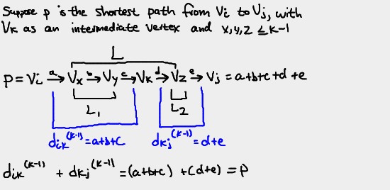
Second scenario

In the second scenario, the k-th vertex, v_k, is in the list of intermediate vertices L. Since we've explicitly stated that the graph contains no negative cycles, we can conclude that v_k occurs in L only once for the shortest path. Otherwise, the second occurrence of v_k would imply an unnecessary cycle -- the path could not possibly be the shortest possible path. Consequently, we can split L into three groups: L1, a list of vertices <= k-1 (since v_k only appears once in L), v_k, and L2, another list of vertices <= k-1. Finally, we conclude that candidates for the shortest path from v_i to v_j are of the form v_i, L1, v_k, L2, v_j.

With this information, we can conclude a couple of things. First, note that above we've shown that there exist paths from v_i to v_k with all intermediate vertices <= k-1. The shortest of these paths by definition is equal to d_ik^(k-1). Similarly, we've also shown there exist paths from v_k to v_j with all intermediate vertices <= k-1. The shortest of these paths by definition is equal to d_kj^(k-1). Since the shortest path from v_i to v_k is d_ik^(k-1) and the shortest path from v_k to v_j is d_kj^(k-1), we can conclude the shortest path from v_i to v_j is (d_ik^(k-1) + d_kj^(k-1))

What we've shown

We've just shown for both cases (v_k in L and not in L) that we can express d_kj^(k) in terms of d_kj^(k-1). The first scenario tells us that as we increase the k in D^(k), the shortest path from v_i to v_j is guaranteed to remain the same despite this bigger k if the new v_k is not an intermediate vertex in a path from v_i to v_j. This makes sense because by definition, the only paths d_ij^(k) has that d_ij^(k-1) does not are paths that involve v_k as an intermediate vertex.

For example:

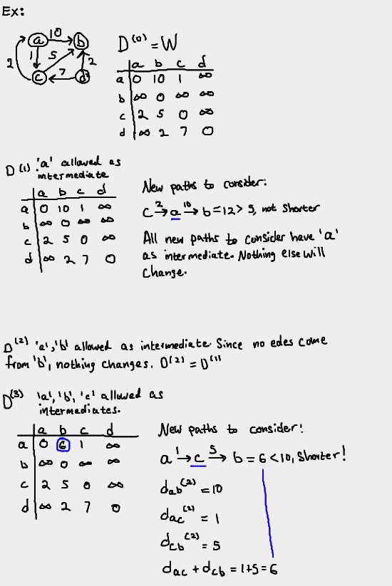
If the introduction of v_k as an allowed intermediate creates new paths from v_i to v_j, then it seems like we would have to calculate the length of all such paths and compare them with eachother to determine the shortest of these new paths, which we'll call p. We would then need to compare p to d_ij^(k-1) to see if this new path is actually shorter than what already existed before the introduction of v_k as an allowed intermediate. However, we already proved that the length of the shortest path that has v_k as an intermediate is exactly (d_ik^(k-1) + d_kj^(k-1)), thus p = (d_ik^(k-1) + d_kj^(k-1)). This reduces our work load to simply comparing p with d_ij^(k-1), and choosing the smaller of the two as the shortest path from v_i to v_j.

This gives us the information we need to finally construct an algorithm.

Algorithm

d_ij^(k) = min{(d_ik^(k-1) + d_kj^(k-1)), d_ij^(k-1)} for k>=1. d_ij⁽⁰⁾ is just the weight matrix.

Pseudocode

This pseduocode overwrites the matrix D each iteration, unlike the Warshall algorithm from part 1. This is more space efficient than keeping track of multiple multiple matrices since we only intend on returning the last matrix D⁽ⁿ⁾.

# W is the nxn weight matrix, indexed at 1
def Floyd(W[1..n, 1..n]):
    D = W
    for k = 1 to n do
        for i = 1 to n do
            for j = 1 to n do
                D[i,j] = min{D[i,j], D[i,k]+D[k,j]}
    return D

Python implementation

The example weight matrix in the implementation represents the following graph, shown earlier in the notes:

 1
 2
 3
 4
 5
 6
 7
 8
 9
10
11
12
13
14
15
16
17
18
19
20
21
22
23
24
25
26
27
28
29

import sys
import copy
INF = sys.maxint # use max_int as 'infinity'

def floyd(W, n):
    D = copy.deepcopy(W)
    k = 0
    while k < n:
        i = 0
        while i < n:
            j = 0
            while j < n:
                D[i][j] = min(D[i][j], D[i][k] + D[k][j])
                j += 1
            i += 1
        k += 1
    return D



# weight matrix of the graph used through the examples in the notes.
W = [
    [0,INF,3,INF],
    [2,0,INF,INF],
    [INF,7,0,1],
    [6,INF,INF,0],
]

print(floyd(W, 4))

raw source

Analysis

Similar to Warshall's algorithm, the time efficiency of Floyd's algorithm is O(n³).

Next time

Next time, we'll apply dynamic programming concepts to searching and optimal binary search trees.

(This post is part of the dynamic programming series.)